Logistic regression is yet another technique borrowed by machine learning from the field of statistics. It’s a powerful statistical way of modeling a binomial outcome with one or more explanatory variables. It measures the relationship between the categorical dependent variable and one or more independent variables by estimating probabilities using a logistic function, which is the cumulative logistic distribution.
The general mathematical equation for logistic regression is −
y = 1/(1+e^-(a+b1x1+b2x2+b3x3+...))
Following is the description of the parameters used −
- y is the response variable.
- x is the predictor variable.
- a and b are the coefficients which are numeric constants.
The function used to create the regression model is the glm() function.
Syntax
The basic syntax for glm() function in logistic regression is −
> glm(formula,data,family)
Description of the parameters used −
- formula is the symbol presenting the relationship between the variables.
- data is the data set giving the values of these variables.
- family is R object to specify the details of the model. It’s value is binomial for logistic regression.
Example
Loading Data
The in-built data set mtcarsdescribes different models of a car with their various engine specifications. In mtcars data set, the transmission mode (automatic or manual) is described by the column am which is a binary value (0 or 1). We can create a logistic regression model between the columns “am” and 3 other columns – hp, wt, and cyl.
> df <- mtcars
> df <- df[,c(9,2,4,6)]
> head(df)
                  am cyl  hp    wt
Mazda RX4          1   6 110 2.620
Mazda RX4 Wag      1   6 110 2.875
Datsun 710         1   4  93 2.320
Hornet 4 Drive     0   6 110 3.215
Hornet Sportabout  0   8 175 3.440
Valiant            0   6 105 3.460
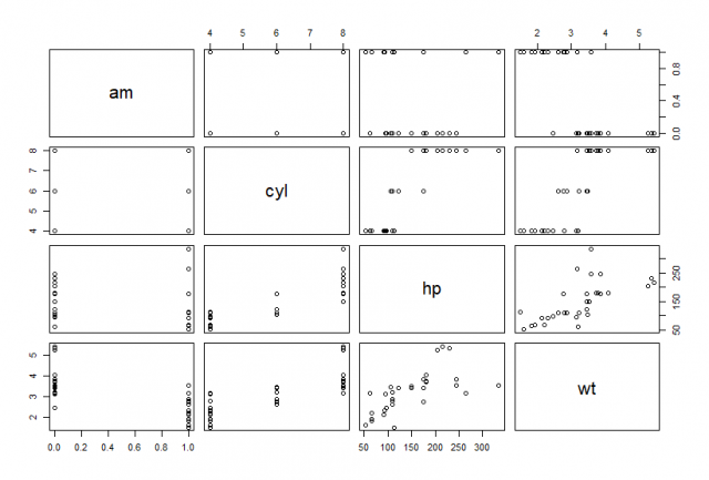
Visualizing Data
Data visualization is perhaps the fastest and most useful way to summarize and learn more about your data.
> plot(df)
Regression Model
We use the glm() function to create the regression model and get its summary for analysis.
> model <- glm(am ~ cyl + hp + wt, df, family=binomial)
> model

Call:  glm(formula = am ~ cyl + hp + wt, family = binomial, data = df)

Coefficients:
(Intercept)          cyl           hp           wt
   19.70288      0.48760      0.03259     -9.14947

Degrees of Freedom: 31 Total (i.e. Null);  28 Residual
Null Deviance:      43.23
Residual Deviance: 9.841        AIC: 17.84
Next, we can do a summary(), which tells you something about the fit:
> summary(model)

Call:
glm(formula = am ~ cyl + hp + wt, family = binomial, data = df)

Deviance Residuals:
     Min        1Q    Median        3Q       Max
-2.17272  -0.14907  -0.01464   0.14116   1.27641

Coefficients:
            Estimate Std. Error z value Pr(>|z|)
(Intercept) 19.70288    8.11637   2.428   0.0152 *
cyl          0.48760    1.07162   0.455   0.6491
hp           0.03259    0.01886   1.728   0.0840 .
wt          -9.14947    4.15332  -2.203   0.0276 *
---
Signif. codes:  0 '***' 0.001 '**' 0.01 '*' 0.05 '.' 0.1 ' ' 1

(Dispersion parameter for binomial family taken to be 1)

    Null deviance: 43.2297  on 31  degrees of freedom
Residual deviance:  9.8415  on 28  degrees of freedom
AIC: 17.841

Number of Fisher Scoring iterations: 8
Conclusion
Hence, we saw how to build logistic regression models using the glm() function and setting family to binomial. glm() does not assume a linear relationship between dependent and independent variables. Also as the p-value in the last column is more than 0.05 for the variables “cyl” and “hp”, we consider them to be insignificant in contributing to the value of the variable “am”. Only weight (wt) impacts the “am” value in this regression model.
This brings the end of this Blog. We really appreciate your time.
Hope you liked it.
Do visit our page www.zigya.com/blog for more informative blogs on Data Science
Keep Reading! Cheers!
Zigya Academy
BEING RELEVANT
