Since income is either consumed or saved, therefore, consumption + saving is always equal to income. It implies that consumption and saving curves representing consumption and saving functions are complementary. Thus given the income, we can derive saving function directly from consumption function as shown in Fig,comprising Part A showing consumption function and Part B showing saving function.
In Part A of the adjoining Fig, CC curve shows consumption function corresponding to each level of income whereas 45° line OL represents income. The 45° line divides the graph in two equal parts and so each point on this line is equidistant from X-axis and Y-axis. CC curve intersects 45° line OL at point B at which BR = OR, i.e., consumption = income. Therefore, point B is called breakeven point. There is no saving at point B but to its left, consumption function lies above 45° line showing negative saving (dissaving) whereas to the right of point B, consumption function lies above 45° line showing positive saving.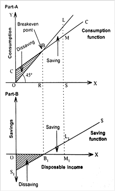
Now in Part B, we derive saving function in the form of saving curve. Remember in Part A, amount of saving (or dissaving) is the vertical distance between CC curve and 45° line. By plotting in Part B of the Figure vertical distances of part A representing saving/ dissaving and by joining them, we derive a saving curve. For instance, (i) at 0 (zero) level of income in Part A, vertical distance OC (representing dissaving) is plotted as OS1 in Part B. Similarly, (ii) at OR level of income in Part A, vertical distance between CC curve and 45° line at point B which is nil (indicating zero saving) is shown as point Bj at the same level of income in Part B. Likewise (iii) at OS level of income, LM vertical distance of Part A is shown as L1M1 in Part B. By joining points St, Bt, Lv we get saving curve. Thus saving function is diagrammatically derived from consumption function in the form of saving curve. (In the same way consumption curve can be derived from saving curve.)


